Hopfield Networks Is All You Need (sic) - Part I | Blum's Blog

Hopfield Networks Is All You Need (sic) - Part I

10 August 2020

Transformers are all the rage nowadays - they’ve made huge strides in many tasks, including enabling the massively successful language model, GPT-3. Hopfield networks, invented in 1974 and popularized in the 80s, are largely considered to be old news. However, they’re not as different as you might think. This post lays the groundwork of understanding for how Hopfield networks function.

Authors

Huberet Ramsauer (PhD Candidates, JKU - Institute for Machine Learning)
Bernhard Schäfl (MSc, JKU - Institute for Machine Learning)
Johannes Lehner (Univ. Prof, JKU- Institute for Organization?)
Philipp Seidl (JKU)
Michael Widrich (Research Asst., JKU - Institute for Machine Learning)
Lukas Gruber (MSc, JKU - Institute for Machine Learning)
Markus Holzleitner (Research Staff, JKU - Institute for Machine Learning)
Milena Pavlovic (Research Fellow, Univ. Oslo - Dept. of Biomed Informatics, Immunology)
Geir Kjetil Sandve (Assoc. Prof., Univ. Oslo - Dept. of Biomed Informatics)
Victor Greiff (Assoc. Prof., Univ. Oslo - Greiff Lab)
David Kreil (Founding Director, IARAI)
Michael Kopp (Founding Director, IARAI)
Günter Klambauer (Asst. Prof, JKU - Institute for Machine Learning)
Johannes Brandstetter (Asst. Prof, JKU - Institute for Machine Learning)
Sepp Hochreiter (Univ. Prof, JKU - Institute for Machine Learning)

ArXiV: https://arxiv.org/pdf/2008.02217.pdf

Background

I’ll be honest, when I came across this paper, I definitely needed a refresher on the details of Hopfield networks. The goal of this article is going to be to give you a high-level understanding of the fundamentals of how Hopfield networks work so, if you’re already familiar, you can skip this post - the next two posts will discuss the paper itself. If you’re looking for a more in-depth review of the topic, I recommend lectures 20 and 21 of CMU’s deep learning course, found here and here.

Hopfield networks can be viewed as content-addressed memory - a way to remember data and then look it up again by giving it data similar to what it remembers. At the highest level, Hopfield networks are defined by an energy function \(E(\vec{\xi})\), which is implicitly also a function of what can be thought of as its stored memory \(X\). To use a network, you input your query \(\vec{\xi}\), and the network changes it in to a different \(\vec{\xi^*}\) which has lower energy. Hopefully this \(\vec{\xi^*}\) corresponds to one of the elements in memory. We’ll see how this works in a little bit more detail below.

Core Idea

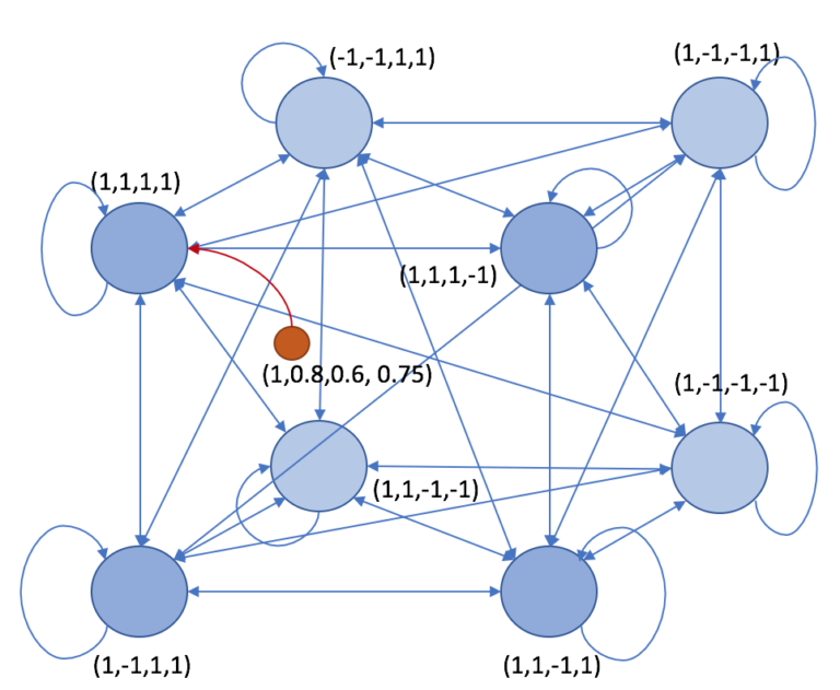
In the traditional formulation, a Hopfield network is a collection of weights connecting nodes. Weights connect each node to each other node and all the weights are symmetric (so node \(i\) has the same weight towards \(j\) as \(j\) does towards \(i\)). Crucially, and in contrast with most neural networks, all the inputs to the network are assumed to be binary, either +1 or -1. To query the network, the nodes are set to the values of the query, \(\vec{\xi_0}\). At each timestep, the algorithm selects a random node and updates its value based on the values of the other nodes. Eventually, the values will stop changing and this can be viewed as the value returned by the query.

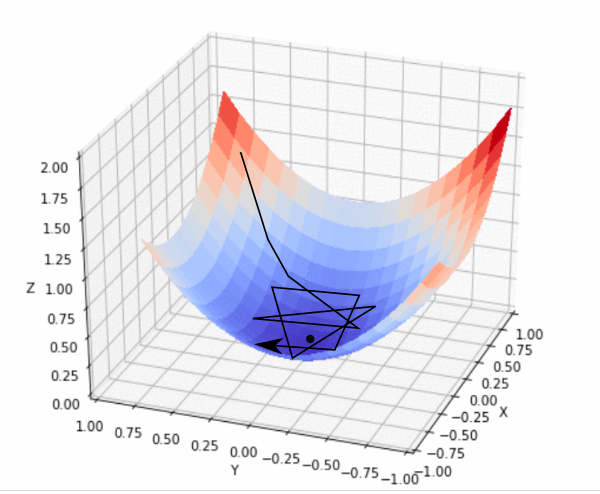
This process is characterized by the energy function, \(E\). Whenever we consider flipping the state of a node, we flip it iff flipping it would decrease the total energy of the system. As a result, when there are no states that could be flipped to achieve a lower energy, the algorithm has reached a stable point. Similar to gradient descent, we can think of the point that we stabilize at as a local minimum of the energy function. Now that we have a function that converges to some value, the only thing left to do is to make sure that it converges to something useful! The entire process is very similar to gradient descent on \(\vec{\xi}\) using \(E(\vec{\xi})\) as the loss function, except that we are doing the entire process in binary and we are changing the values of the nodes instead of the weights.

So, now we have established a process that converges to something, we just have to rig it so that it converges to something useful.

Details

In the classic version, the energy function is given by :

\[E(\vec{\xi}) = -\sum_i \xi_i (\sum_{j \neq i} 0.5 w_{ij} \xi_j + b_i)\]

Our goal is to only flip a bit when it would reduce the total energy of the system. If \(\xi^{t+1}\) is \(\xi^{t}\) with the \(i^{th}\) bit flipped, then we can derive the difference between the energy functions :

\[E(\vec{\xi^{t+1}}) - E(\vec{\xi^{t}}) = -\sum_i (\xi^{t+1}_i - \xi^{t}_i) (\sum_{j \neq i} w_{ij} \xi^t_{j} + b_i)\]

Notice that we got rid of the 0.5 because we double-count each weight. For all \(i \neq j\), \((\xi^{t+1}_i - \xi^{t}_i ) = 0\) because we’re only changing one bit. We want to flip the bit so that \(E(\vec{\xi^{t+1}}) - E(\vec{\xi^{t}}) \leq 0\) (i.e., our energy is decreasing). Looking at the above sum, we can see that it is 0 if we do not change and it is negative iff the sign of \(\xi^{t+1}_i - \xi^{t}_i\) matches the sign of \((\sum_{j \neq i} w_{ij} \xi^t_{j} + b_i)\). Whenever we can make this term negative, it will decrease the energy of our system, and we want to flip the value. We can formalize this as our update rule in vector notation:

\[\xi_i^{t+1} \leftarrow \theta(\vec{w_{i}} \vec{\xi^{t}} + b_i)\]

where \(\theta\) is the sign function, \(w_{i}\) is the \(i^{th}\) row of \(W\) (our weight matrix) and \(\xi\) is represented as a column vector. (Note: here, we assume that \(W_{i,i}=0\)). While the classic version updates individual nodes one at a time, we could just as easily update all nodes in \(\xi\) at once, letting us rewrite our update function in matrix notation:

\[\xi_i^{t+1} \leftarrow \theta(W\vec{\xi^t}+\vec{b})\]

When this update rule reaches a fixed point, we have converged. Notably, if we fix \(W := (\xi^t)^T(\xi^t)\) and \(b := \vec{0}\), we will be guaranteed a fixed point at \(\xi^{t}\). More generally, if we have a set of vectors \(X = \{\xi_0, \xi_1, ..., \xi_n\}\) that we want to remember, setting \(W := X^TX\) and \(b := \vec{0}\) will result in a fixed point at each of the memory vectors \(\xi_{0..n}\). This strategy of setting \(W\) is called the Hebbian Learning Rule. We can ‘remember’ more memories by simply adding them to \(X\) and updating \(W\).

In general, there are other choices that you can make for how to set \(E\), which will in turn induce different update rules and different schemas for assigning the weights, but they all follow this broad framework.

Limitations

Below are some limitations of the Hopfield networks we talked about, in no particular order.

Hopfield networks only take in binary data in the form of \(\pm 1\)
The ‘memory’ that the network converges to is not necessarily what you would consider to be the closest.
There exist metastable states, which are states that are NOT memories but are still points that the network can converge to
It takes \(O(n^2)\) time to update all \(n\) nodes each iteration, and multiple iterations are usually needed to converge
In the traditional formula, the network can only ‘memorize’ \(~0.14n\) different patterns before problems start emerging
Hopfield networks can often struggle if the patterns are not well-separated

General Thoughts

Hopfield networks are an interesting method for content-addressable memory, with some strong theory behind them (google it- there’s always more to read). That being said, they also have some pretty severe limitations that hamstring their applicability. Because of this, they eventually gave rise to Boltzmann machines, a similar model that attempts to move past some of these limitations. However, in the next post, we won’t be focusing on Boltzmann machines. Instead, we’ll take a look at a modern (and very influential) instance of Hopfield networks - Transformers!