Hopfield Networks Is All You Need (sic) - Part II
12 August 2020
Transformers are all the rage nowadays - they’ve made huge strides in many tasks, including enabling the massively successful language model, GPT-3. Hopfield networks, invented in 1974 and popularized in the 80s, are largely considered to be old news. The previous post, found here provided a primer on Hopfield networks. In this post, we’ll explore the connections between transformer models and Hopfield networks.
Authors
- Huberet Ramsauer (PhD Candidates, JKU - Institute for Machine Learning)
- Bernhard Schäfl (MSc, JKU - Institute for Machine Learning)
- Johannes Lehner (Univ. Prof, JKU- Institute for Organization?)
- Philipp Seidl (JKU)
- Michael Widrich (Research Asst., JKU - Institute for Machine Learning)
- Lukas Gruber (MSc, JKU - Institute for Machine Learning)
- Markus Holzleitner (Research Staff, JKU - Institute for Machine Learning)
- Milena Pavlovic (Research Fellow, Univ. Oslo - Dept. of Biomed Informatics, Immunology)
- Geir Kjetil Sandve (Assoc. Prof., Univ. Oslo - Dept. of Biomed Informatics)
- Victor Greiff (Assoc. Prof., Univ. Oslo - Greiff Lab)
- David Kreil (Founding Director, IARAI)
- Michael Kopp (Founding Director, IARAI)
- Günter Klambauer (Asst. Prof, JKU - Institute for Machine Learning)
- Johannes Brandstetter (Asst. Prof, JKU - Institute for Machine Learning)
- Sepp Hochreiter (Univ. Prof, JKU - Institute for Machine Learning)
ArXiV: https://arxiv.org/pdf/2008.02217.pdf
Background
If you haven’t read the previous post in this sequence or are unfamiliar with Hopfield networks, I recommend you read that here first. We covered the traditional formulation of Hopfield networks, which take operate on vectors of binary values (\(\pm 1\)) and use the energy function
\[E(\vec{\xi}) = -0.5 \vec{\xi}^T W \vec{\xi}\]for a query column vector \(\vec{\xi}\) and \(W := X^TX\), where the rows of \(X = \{\vec{x_0}, \vec{x_1}, ..., \vec{x_n}\}\) correspond to the memories/patterns stored in the network. This corresponds to the following update rule :
\[\vec{\xi}^{t+1} = f(\vec{\xi}^t, X) = \theta(W\vec{x}_i^t + \vec{b}) = \theta(X^TX\vec{\xi}^t)\]Fast forward to modern day, a more common energy function is \(E(\vec{\xi})\) is \(E(\vec{\xi}) = -\sum_i \exp (\vec{\xi}x_i^T)\). They can now store \(2^{n/2}\) patterns of length \(n\), but they still only operate on binary data. The authors of this paper propose a simple but impactful change - changing the Hopfield networks to operate on continuous data (and updating the associated energy function).
Core Idea
The big idea of this paper is that we can choose an energy function that makes the update rule of the Hopfield net the same as a forward pass of a transformer layer!
The authors also provided some interesting experiments of existing transformer models in their experiments.
The authors sum up their changes pretty well in a single graphic :

For reference, the \(\text{lse}\) and \(\text{softmax}\) equations are defined as follows:
I wrote the energy function in a slightly different way from the graphic, but it’s easy to check that they reduce to the same thing.
You might have noticed that the new energy function is very similar to the old one : it’s the log of the old energy with some other terms added. The \(c\) isn’t important, but the \(\vec{\xi}^T\vec{\xi}\) is : it constrains the values of \(\vec{\xi}\) so that they don’t grow to infinity (which wasn’t a problem with the old networks, as they only used \(\pm 1\)).
The final thing to note is the last box. I’ll assume working knowledge of transformers - if you aren’t famimliar with them, there are a bunch of excellent tutorials on the internet. The thing here to note is that the update rule for our continuous Hopfield net is extremely similar to a forward pass of an attention module.
In fact, if you just set \(\beta := \frac{1}{\sqrt{d_k}}\), let \(\vec{\xi}\) be our query (you can even put them together in to a matrix \(Q\)) and let our memorized patterns \(X^T\) to be the keys, we’ve basically recovered the exact same equation. The one thing to note is that the update equation shown sums over (the equivalent of) the keys - \(X\) - instead of the values. In real-life transformers, the keys and the values are often the same thing anyways, but if you want to encode them, you can just multiply the keys, queries and values by encoding matrices.
Details
If you like math, there’s a lot of exhaustive math in the appendix of this paper that I recommend you look at it. I won’t cover it here, but it’s all very well proven. Instead, I’ll try to repeat key takeaways from this section of the paper.
- This process always converges : If you treat these layers as hopfield layers, you’ll always converge to some value \(\vec{\xi}^*\) regardless of the \(\vec{\xi}\) you put in. \(^\dagger\)
- This process converges exponentially : Each time you update, the difference between your current energy \(E(\vec{\xi})\) and the target energy \(E(\vec{\xi}^*)\) decreases by some factor \(k\).
- The number of keys you can grows exponentially as you add more dimensions : The base of the exponent, how fast it grows, is based on how well-separated the keys are, how much error you’re willing to accept, how many dimensions you have and how large of an area your keys are sampled from.
- If the patterns aren’t well-separated, it’s possible to get global fixed point : This means that no matter what you put in, you get the same result (after enough iterations).
\(^\dagger\) Note: Technically it can converge to a compact set of values that all have the same energy.
Experiments
The authors also provide some graphics looking at BERT models (used for language modeling) through the lens of Hopfield networks.
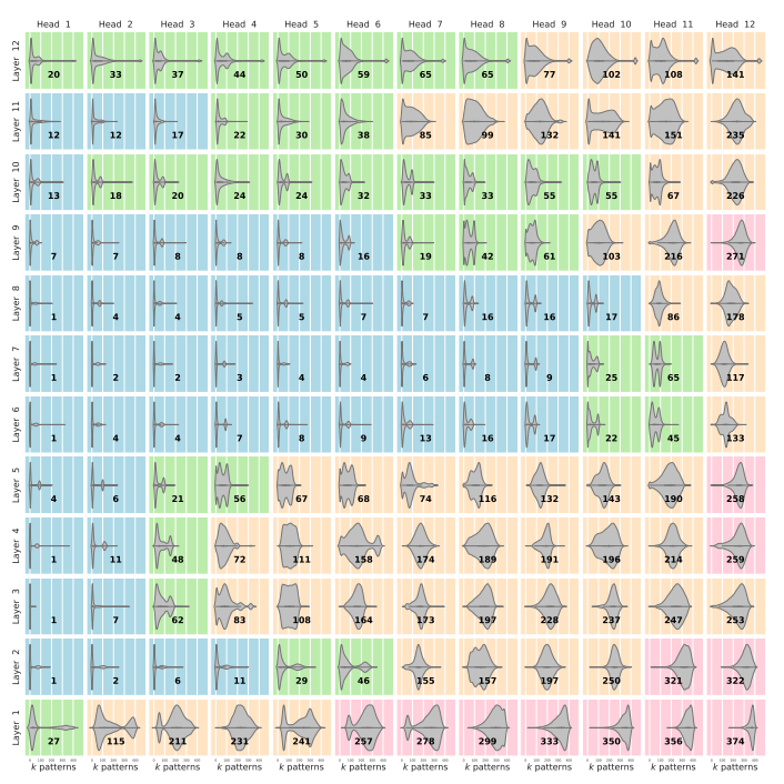
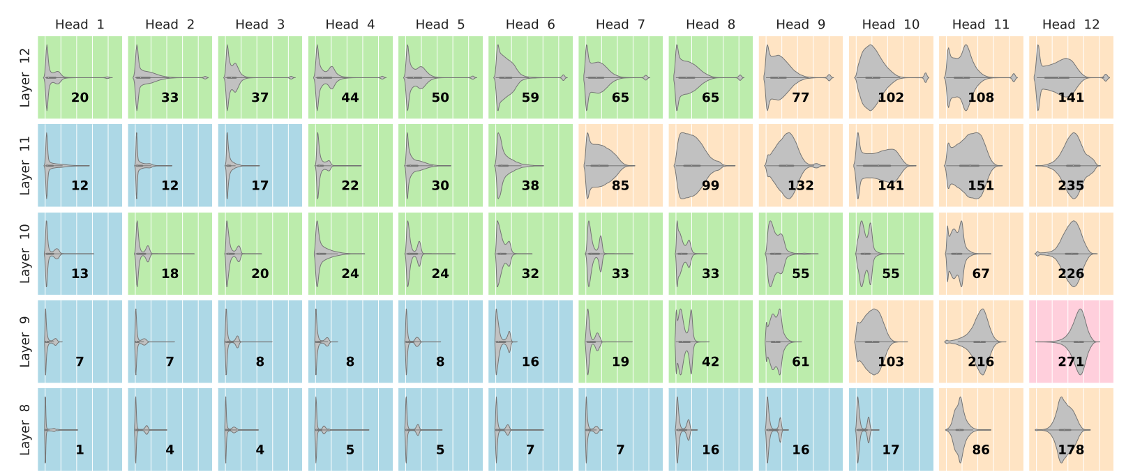
First, they plot how widely the attention is spread among the inputs to each head:

For each head, a histogram is provided of how many nodes are needed to account for 90% of that head's attention
For a brief key, red corresponds to very broad attention, orange: somewhat broad attention, green: somewhat focused attention, blue: very focused attention.
The authors note that most of the heads in the input layers have very broad attention, while the layers in the middle have very focused attention.
In the language of Hopfield networks, a broad attention corresponds to a metastable point - a stable point that is a mixture of different memories.
The authors provide a variety of hypotheses as to why these behaviours are what they are, and I think that confirming or disproving those hypotheses could be interesting research directions.
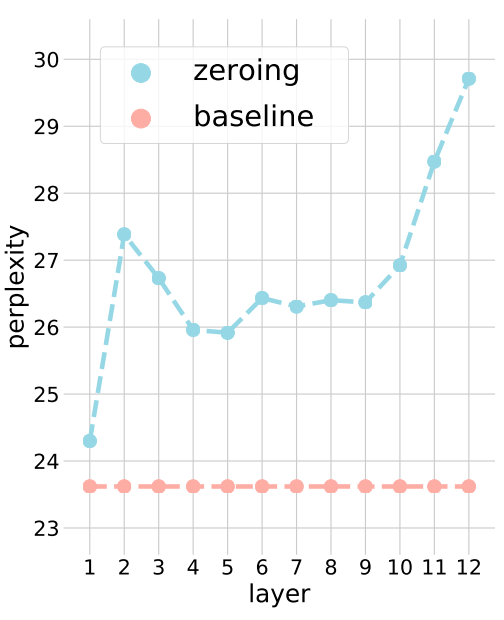
Among them, they note that the initial layers basically just perform averaging, so they propose literally replacing the initial layers with a mask that does averaging :

Surprisingly, you can basically replace the first layer, but you definitely shouldn't get rid of the later ones
They evaluate the modified model evaluated on a language task where perplexity is a measure of error.
Notably, the perplexity doesn’t go up much at all when replacing the first layer, but it skyrockets when we get rid of the later layers.
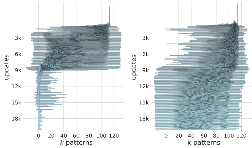
Perhaps most intriguingly, the authors observe that most of the layers perform simple averaging for the first several thousand iterations, but the loss starts to decrease very suddenly when they all start breaking away from this behaviour.

In experiments performed on small BERT models, the behaviour is very stark

The attention for two sample heads in intermediate layers continually decreases as training continues
The authors also have a companion paper evaluating the Hopfield layers on some biological datasets, but I’ll skip that for now.
Future Directions
The authors provide a nice plug-and-play implementation of their code at https://github.com/ml-jku/hopfield-layers.
More generally, this paper helps build a solid theoretical understanding of transformers. In particular, the part that I see with the most impact going forward is probably the data analysis of existing models. Understanding the layout of the metastable points in transformer models opens up a lot of questions. For instance,
- If learning goes a lot faster when some of the layers start focusing their attention more, could we speed up the process by initializing the attention layers to values that result in highly discriminative attention?
- Are the layers with broad attention not done learning? Are they redundant? Could they all be replaced with averaging? Or do they serve another purpose?
- Alternately, are the layers with broad attention more specifically paying attention to everything EXCEPT a couple of inputs?
- If the layers are truly just performing averaging, what value does that add? Perhaps the value is instead being added in the encoding of the values, in which case they could be replaced with linear layers
On the topic of Hopfield networks, this opens up the question of whether or not lessons learned in designing energy functions in Hopfield networks could be used to design better models that are similar to attention? I don’t personally know enough about the existing body of work in this area to answer that question, but I’m sure there must be something.
General Thoughts
This paper was really well-done on pretty much all axes. While it was quite dense and difficult to read, it has multiple contributions to the field and the math is proven extremely rigorously. Hopefully it spurs more interest in resurrecting Hopfield networks in general. I thoroughly recommend reading the paper itself for anyone interested in the topic!
