Never Give Up: Learning Directed Exploration Strategies
17 August 2020
One of the hardest topics in reinforcement learning is exploration, choosing which things are worth trying. Some methods try to avoid visiting states twice in the same episode, while others try to diversify exploration over the life of the training process. DeepMind’s “Never Give Up” algorithm tries to do both.
Authors
- Adria Puigdomenech Badia (Res. Eng. - DeepMind)
- Pablo Sprechmann (Res. Sci. - DeepMind)
- Alex Vitvitskyi (Res. Eng. - DeepMind)
- Daniel Guo (Res. Sci. - DeepMind)
- Bilal Piot (Res. Sci. - DeepMind)
- Stephen Kapturowski (Res. Eng. - DeepMind)
- Olivier Tieleman (Res. Sci. - DeepMind)
- Martin Arjovsky (MILA?)
- Alexander Pritzel (Sen. Res. Sci. - DeepMind)
- Andrew Bolt (DeepMind)
- Charles Blundell (Sen. Res. Sci. - DeepMind)
ArXiV: https://arxiv.org/pdf/1810.02338.pdf
Background
Many methods have recently been providing either episodic or lifelong exploration rewards. Each have their downsides : episodic rewards can forget everything else that the agent has done before this episode, while lifelong exploration strategies can be veerrryy slow to adapt. (As a side note, the episodic exploration strategies tend to also scale poorly with the number of memories in the memory buffer). This could result in the agent trying the same thing many times before learning that it’s futile. Either way, these strategies usually work by taking the extrinsic reward \(r^e\) (reward from the environment) and adding intrinsic reward \(r^i\) to it.
Core Idea
As noted above, there are two big parts to their method : the episodic and lifelong exploration bonuses
Episodic Exploration
This paper’s primary contribution is their choice of intrinsic reward. Like many papers, their goal is to reward new observations that the agent hasn’t seen yet this episode. One classic version of this is count-based exploration : give each state \(s\) an additional reward \(\frac{1}{\sqrt{n(s)}}\), where \(n\) is the number of times that state \(s\) has already been visited. However, this classic has a couple of obvious problems. 1. It requires you to maintain a count of observations of ALL previous memories 2. It doesn’t penalize observations that are similar, but not exactly the same as, previous observations/memories.
This paper partially addresses the first problem by only comparing with memories from the current episode. For the second one, it uses a distance function. First, it learns a siamese network, which implicitly embeds the states in a space where irrelevant information is dropped. Both the episodic memories and the current observation are embedded with this. Then, it calculates the Euclidean distance between the embedding of the current state \(s\) and all of the previous states. It aggregates these all together to get an approximation of \(n(s)\).
Lifelong Exploration
The authors use Random Network Distillation (RND) for their lifelong exploration bonus (if you’re familiar with it, you can skip this - otherwise, keep reading). For RND, the authors initialize a CNN to random weights - this is the random network and we’re never actually going to train it. Instead, we try to have a second network predict the outputs of this network. Intuitively, you can think of the random network as a random function, and the second network is trying to learn this random function. On areas of the data that it’s seen before, the second network should have pretty low error, whereas it’s likely to do less-well on areas that it hasn’t seen before. If you squint hard enough, you can kind of see the error of the second network on some datapoint \(x\) as an inverse distance function from the data points it has seen in its training set.
Following this logic through to the end, and you can train the second network using the agent’s previous observations as input (and the first network as a target output).
Then, when the agent visits state \(s\), you can give the agent a bonus equal to the second network’s error on \(s\), because the error will be higher the more ‘novel’ \(s\) is.
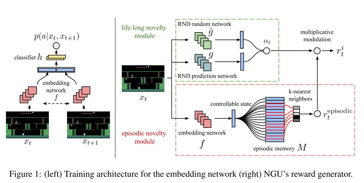
The author-provided schematic of their algorithm is below :
Details
Unfortunately, there are a fair number of details, so I’ll try to highlight the most important ones.
- Siamese Network: Given the triple \(\{o_t, a_t, o_{t+1}\}\), the siamese network tries to predict \(a\) using a network of the form \(f(e(o_t), e(o_{t+1}))\), where \(e\) is the encoding.
- Distance Function: The ‘distance’ between two observations \(o_t\) and \(o_i\) is given by \(d(o_t, o_i) = \|e(o_t)-e(o_i)\|_2\), where \(\|\cdot\|_2\) is the euclidean norm.
- Similarity Function: The similarity between those two observations is then \(K(o_t, o_i) = \frac{\epsilon}{\frac{d(o_i, o_t)}{d_m} + \epsilon}\). \(\epsilon\) is just a small number, like \(10^{-3}\) for numerical stability. \(d_m\) is the running mean of the distance to the \(k^{th}\) nearest observation. Intuitively, this function scales between 0 for very high distances and 1 when there is no distance.
- Unclipped Reward: \(r^{episodic} = \frac{1}{\sqrt{\sum_{i} K(o_t, o_i)} + \epsilon}\). If you see \(K\) as a soft version of equality, then this is similar to the \(1/\sqrt{n}\) equation we saw earlier, with \(\epsilon\) added again because numerical stability is unfortunately a thing.
- Scaled Reward: The authors scale this reward by \(\alpha_t\), which controls how important the bonus is. This value is clamped between \(1\) and \(L\), where \(L\) is another hyperparameter.
- Lifelong Reward: Let \(g\) be the random network and \(\hat{g}\) be the approximator (second) network. Then \(\text{err}(o_t) = \|g(o_t) - \hat{g}(o_t)\|\), and the reward is given by \(1 + \frac{\text{err}(o_t) - \mu_e}{\sigma_e}\), where \(\mu_e\) and \(\sigma_e\) are the running mean/SD for the error.
- The intrinsic rewards can be slowly decreased over time, with a weight of \(0\) amounting to the greedy policy.
The authors train their agent using the R2D2 algorithm from ‘Recurrent Replay Distributed DQN’ to train their algorithm. They use the retrace loss function. I might cover these two algorithms in the future, but it’s enough to think of them as somewhat black boxes for now, with the caveat that it trains multiple agents with different hyperparameters and shares their memory is \(N\) mixtures.
Experiments
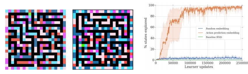
The authors provide a toy experiment in an environment they call the ‘random disco maze’, where the walls of the maze are different colors. Their primary result is a comparison with several other algorithms on Atari games. They separate these in to two categories - ‘hard exploration’ games (really just Montezuma’s Revenge and Pitfall) and ‘dense reward’ games. They primarily provide ablation studies against their own algorithm without various components, with \(R2D2\) representing both the lifelong and episodic intrinsic rewards removed.
The results are shown here:
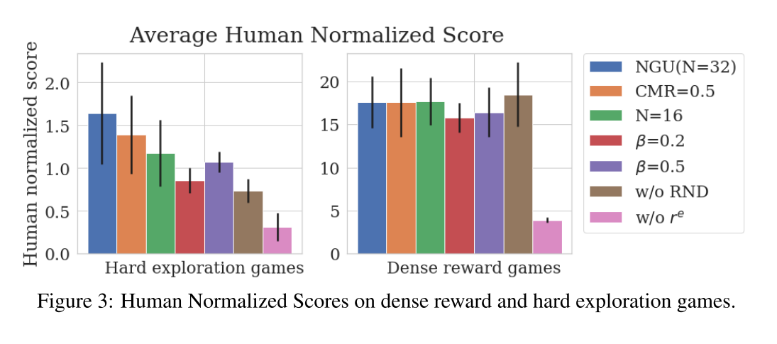
Unsurprisingly, the algorithm doesn't work so well when you remove the extrinsic rewards (pink)
For reference, \(\beta\) corresponds to how heavily the extrinsic rewards are weighted. It looks like their algorithm is fairly resilient to hyperparamter tuning on the ‘easy’ (dense) games, but that could also just be because their algorithm isn’t doing much.
On the hard games, it’s much less stable. The authors provide some additional ablations, which give a similar story.
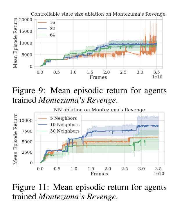
The top graph shows what happens when you change the size of the encoding. Bottom graph shows what happens if you use different values of kth nearest neighbor when calculating similarities.
The authors don’t include other curiosity metrics, which is slightly suspect to me.
Future Directions & General Thoughts
The core idea here is good : explore states that are less similar to states you’ve already seen, and combine lifelong and episodic exploration policies. That being said, I’m not convinced that this is the best path forward. Their episodic memory algorithm takes \(O(n)\) time for each timestep, where \(n\) is the number of timesteps in the current episode - I just can’t see that working for something like DOTA or Starcraft (or worse, real-life). There are also a lot of hyperparameters here, and it looks like they can be relevant. I think having more hyperparameters hurts the democratization of AI, as people with limited compute can’t afford to try all of them. Even for those who can, doing grid-based hyperparameter sweeps increases exponentially in cost with the number of hyperparameters. Finally, you have to manually turn down exploration as the agent converges, which is just not theoretically satisfying.
I actually have an idea that I’ve started working on that’s related to some of these criticisms, hopefully I’ll have a snippet explaining the motivation up soon!