Neural Episodic Control
22 August 2020
In this paper, we again talk about one of reinforcement learning’s favorite topics - why is RL so glacially slow????? The authors provide a number of hypotheses as to why this may be the case and then propose a model based on non-parametric memory that speeds up learning significantly on a number of tasks. To summarize it in one sentence: what if we estimated the Q-value of new observations to be a weighted sum of the Q-value of similar observations?
Authors
- Alexander Pritzel (Sen. Res. Sci. - DeepMind)
- Benigno Uria (Res. Sci. - DeepMind)
- Sriram Srinivasan (ML Lead - DeepMind)
- Adria Puigdomenech (Staff Res. Eng. - DeepMind)
- Oriol Vinyals (Princip. Sci. - DeepMind)
- Demis Hassabis (CEO - DeepMind, casually)
- Daan Wierstra (Princip. Sci. - DeepMind)
- Charles Blundell (Sen. Staff. Res. Sci. - DeepMind)
ArXiV: https://arxiv.org/pdf/1703.01988.pdf
Background
Although reinforcement learning has shown a lot of impressive results, even achieving super-human performance on most Atari games, it still isn’t widely used in industry. One of the biggest reasons for this is that these models are difficult to train in the real-world. Creating a robot and letting it act in potentially dangerous ways for months to years, just to get a trained RL agent, isn’t an enticing proposition for business leaders. While there are a couple of problems here (safety, transfer from simulation, off-policy learning) one of the biggest ones is the raw amount of data necessary.
The authors suggest a number of reasons for this, ranging from slow learning rates to sparse rewards to slow propagation of rewards. When you divide it like this, It actually provides an interesting look at different areas of RL right now : This method tries to solve the first problem, while exploration methods try to solve the second and hierarchical RL tries to solve the third.
A lot of people are enthused about episodic methods right now, and this paper provides another take on how to implement it. The goal is that we can improve the efficiency of learning by more efficiently reaching back to relevant memories.
Core Idea
Unlike most episodic methods, this paper doesn’t just save all of this episode’s memories in a buffer. Instead, it saves ALL memories that the agent has experienced. When it comes time to make a new decision, the algorithm follows the Q-learning framework, estimating the value of each action, and taking the highest one (OK, it’s technically \(\epsilon\)-greedy).
It does that by reaching back in to memory and selecting similar previous observations. It then takes a weighted sum of all of the Q-values for each of those memories in order to estimate the Q-value of each action at the current state/observation. As I’m sure you’re unsurpised to here, the sum is weighted such that more similar observations in memory are given more weight.
The last question you might have is how are we actually training the Q-values?. Well, we use the typical N-step double DQN method (the authors say this is just what they found to work best). For those who haven’t seen it before, let \(\gamma\) be the standard discount factor and let \(Q^{(N)}\) be some other Q-network, usually a lagging version of the Q-network we’re trying to train.
Our target is then given by
\[Q^{(N)}(s_t,a) = \sum_{i=0}^N \gamma^i R_{t+i} + \gamma^N \max_a Q(s_{t+N}, a)\]If you’ve seen Double DQNs before, this is extremely similar - instead of simply using the immediate reward plus the Q-value (technically V) of the next state, we use the next \(N\) rewards and the Q-value of the state after that. The one thing to note is that, rather than using the default method for calculating Q-values, the Q-value is calculated using this weighted sum strategy. The values in the dictionary can be updated using the classic tabular learning rule:
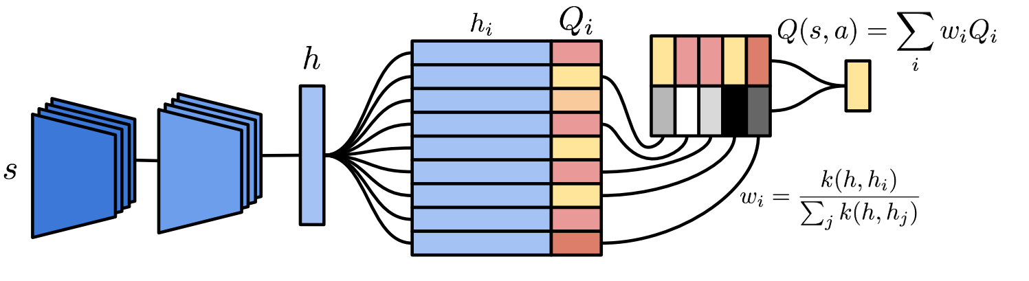
\[Q_i \leftarrow Q_i + \eta (Q^{(N)}_i - Q_i)\]The authors provide the following image to help put it all together.
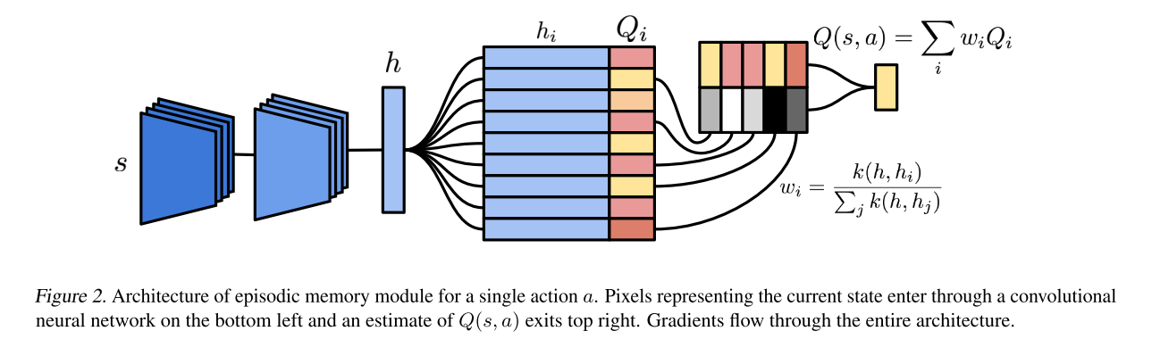
Honestly, the pretty colors make it easier for me, not sure why.
Details
This algorithm was fairly unintuitive to me, so I’ll try to walk through it step by step. Our goal is to derive accurate Q-values, but we have two separate things to learn in this process: the embedding function and the Q-values themselves. I’ll start by talking about how we learn each of these, starting with the Q-values. For the sake of clarity, I’ll differentiate the calculated Q-values as the \(Q^*\) values and the stored ones as Q-values
Whenever we are forced to give a \(Q^*\)-value for state \(s\), either for acting or as a prediction target, we don’t just look it up in the dictionary, nor do we just compute it as a function of the embedding. We begin by calculating the embedding \(h = g(s)\), where \(g\) is our embedding function. We then look to our memory of ALL observations we have ever seen (listed in an embedded form in a KD-tree), and we select the \(k\) nearest neighbors. The authors only use the \(k\) nearest neighbors because they’re not computational masochists (even though they are Google with a metric ton of compute available). The KD-tree actually makes this look up time pretty reasonable (approximately \(log(n)\) in the number of memories, if I recall correctly). We’ll call these selected memories \(m_i\). For each of these nearest memories, we want to calculate their similarity, for which the authors use the inverse kernel.
\[k(h, m_i) = \frac{1}{\|h - m_i\|_2 + \sigma}\]where \(\sigma\) serves her classic role providing numerical stability. Intuitively, this gives a value of \(\frac{1}{\sigma}\) when we have an exact match and roughly \(0\) when two things aren’t even close. The weights \(w_i\) are then these similarity values normalized to sum to 1. Keep this process in mind, it will be useful for training both the Q-values and the embedding.
Now that we have these weights \(w_i\), our calculated \(Q^*\)-value is given by
\[Q^*(s,a) = \sum_i w_i Q(m_i, a)\]The \(Q(m_i, a)\) is simply retrieved from our lookup table, which the authors term the Differentiable Neural Dictionary, because those are all pretty hot words right now and they are accurate. This \(Q^*\) is used for acting and is used as a prediction target. Using the \(Q^*\) nomenclature, I’ll rewrite our update rule, starting with the target \(Q^{(N)}\):
\[Q^{(N)}(s_t,a) = \sum_{i=0}^N \gamma^i R_{t+i} + \gamma^N \max_a Q^*(s_{t+N}, a)\]We then update the value stored in the dictionary. For brevity, let \(Q_i = Q(g(s_t), a)\) and \(Q^{(N)}_i = Q^{(N)}(s_t, a)\) correspondingly.
\[Q_i \leftarrow Q_i + \eta (Q^{(N)}_i - Q_i)\]This updated value is updated in the memory buffer. The authors aren’t very explicit about how the embedding function is trained, but this is my best reconstruction of how they do it. Readers will note that the portion in parentheses is the classical N-step TD-Error. If we replace \(Q_i\) with \(Q^*_i\), we can differentiate this error with respect to the weights. These weights are, of course, functions of the embedding (by way of the inverse kernel), so we can further backprop to the embedding function.
OK, now that we’re done with the hard parts, a couple of notes:
- The authors find that they can actually use pretty high values of \(\eta\) to train their agent, which allows it to learn quickly.
- Whenever the authors run across a key that’s already in the dictionary, they replace the old value rather than add a new entry.
- The rest of the algorithm is trained very similarly to how you would expect, using a replay buffer
Experiments
This post is getting pretty long, so I’ll be fairly brief with the experiments section.
The algorithm performs pretty well , both in terms of final score and learning rate.
Here are a few samples (which I’m sure are cherry-picked, but are promising nonetheless)
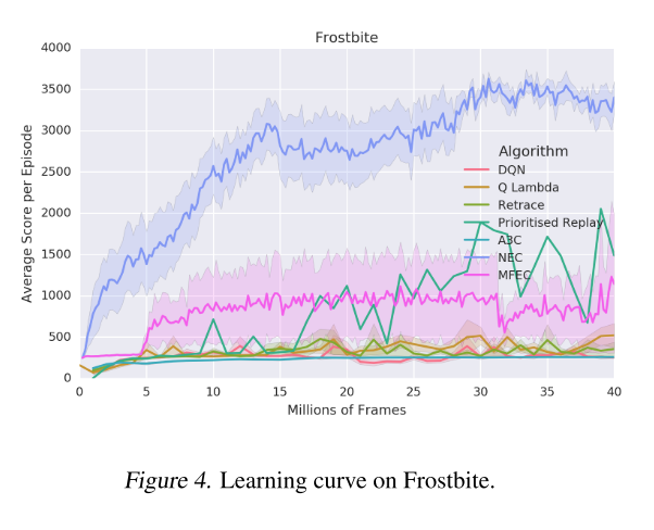
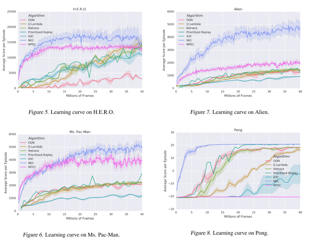
It's not clear whether this algorithm is necessarily learning faster or just achieving a higher score, largely because the other algorithms are doing much worse.
The learning curves provided for the NEC (Neural Episodic Control) algorithm look a lot like a log or sqrt curve, which indicates that it does most of its learning pretty quickly.
To contrast, the other algorithms look like they improve more or less linearly, although it’s hard to tell.
When I looked at the grand table of results in the appendix, it wasn’t as clear that NEC generally outperforms the other algorithms.
In fact, another algorithm MFEC outperformed NEC about as often as NEC outperformed it.
General Thoughts
I think that the most difficult thing with this algorithm is the lack of ablation studies. As you can see from the details section, the algorithm has a lot of new and interesting contributions. That being said, I’m not sure to what degree each of them are actually helping. For instance, how do we know that the embedding network is actually doing anything?
It’s entirely possible that just doing raw pixel similarity gets you most of the performance gains of this method, with a lot less computation and complexity. I’m sure that wouldn’t sell, because that’s just a minor update on the tabular algorithm, which isn’t fashionable. I think that the goal with algorithms should always be to get the greatest results with the most flexibility and the least complexity, so that’s probably worth checking.
Overall, it’s an interesting idea, and I appreciate that they found a way to make it (slightly) more computationally tractable using KD-trees, but I’m not super sold it’s the way forward.