MetaGenRL : Improving Generalization in Meta-Reinforcement Learning Using Learned Objectives
24 August 2020
One interesting aspect of reinforcement learning is that, while the value functions, Q-functions and policies are all learned automatically, the underlying algorithms, such as REINFORCE or Q-learning are not. On a high level, this paper intends to learn a loss function that can be used to train a reinforcement learning agent by using meta learning. Most crucially, it tries to do so on legitimately unrelated tasks, which is a stark departure from existing work.
Authors
- Louis Kirsch (Phd Cand. - IDSIA)
- Sjoerd van Steenkiste (PhD Cand. - IDSIA)
- Juergen Schmidhuber (Prof. - IDSIA, Lugano)
ArXiV: https://arxiv.org/pdf/1910.04098.pdf
Background
In reinforcement learning, most algorithms can broadly be divided into one of two groups : policy-based algorithms (like IMPALA) and Q-value based algorithms (see Rainbow). For the sake of this paper, we’ll focus on policy-based algorithms. The canonical policy-based algorithm is A2C (Advantage Actor Critic), which learns a policy \(\pi_\phi(a|s)\) parameterized by \(\phi\) and an Advantage function \(A_\theta(a|s) = Q(s,a) - V(s)\), parameterized by \(\theta\). As usual, \(s\) and \(a\) are states and actions respectively. Similar to how the discriminator-generator dynamic works in GANs, the critic evaluates \(\pi\)’s actions and is used in its update function :
\[E_{\tau}\Big[\nabla_\phi \sum_{t} \log(\pi_\phi(a_t|s_t))A(a_t, s_t)\Big]\]Given the full trajectory \(\tau\) of length \(t\), one way to compute \(A\) is using the raw reward sample \(A(s_t, a_t) = \sum_{i=0}^{T-i} \gamma^i R_{t+i} - V(s_t)\), we can alternately phrase the advantage function as a function of \(\tau\), \(V\) and \(t\). Similarly, because our trajectory \(\tau\) already includes our actions and states \(t\), we can compute \(\nabla_\phi\log(\pi_\phi(a_t|s_t))\) if we just know \(\phi\), \(\tau\) and \(t\). We can then rewrite this gradient calculation as
\[\nabla_\phi E_{\tau}\Big[\nabla_\phi L(\tau, V, \phi_\phi)]\]where
\[L(\tau, V, \pi_\phi) := \sum_t \log\Big(\pi_\phi(a_t|s_t)\Big) \Big[\sum_{i=0}^{T-i} \gamma^i R_{t+i} - V(s_t)\Big]\]is our loss term. However, this function doesn’t necessarily have to take exactly this form.
Core Idea
The big idea of this paper is that we could learn this loss function just like any other function. Of course, to do this, we need a loss-function for our loss-function (now that’s pretty meta). It’s probably helpful to list some desiderata for our loss function.
- We would like our agent to do better (more reward) after it has been updated using this loss function.
- The loss function should account for the fact that our current decisions affect decisions later down the line.
- Our loss function should be differentiable
In general, we’re not looking to change anything about our original update rule besides \(L\). For a reminder, our initial update rule was \(\phi' = g(L, \phi| \tau, V) = \phi - \eta \nabla_\phi L(\tau, V, \pi_\phi)\). For simplicitly, I’ll drop the \(\tau\) and \(V\) during the explanation.
We can formalize the first desiderata as \(Q_{\phi'}(s,a) - Q_{\phi}(s,a)\). If \(L_\alpha\) is a neural network parameterized by \(\alpha\), we can then train \(L\) to maximize this improvement via gradient ascent (this conveniently fulfills our 3rd requirement).
A schematic of the network is shown below:
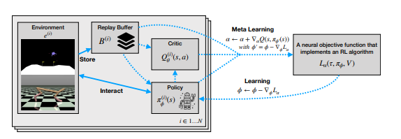
Probably non-trivial to implement
In general, note that \(\phi'\) is dependent on \(L\) and \(\phi\), so that our choices of \(\alpha\) affect the gradient updates on \(\pi_\phi\).
To fulfill our third requirement, we use an RNN that processes the trajectory backwards in time, meaning that, by the time it evaluates a given action, it has already seen the effects of those actions.
Unfortunately, this requires the gradient of a gradient to be computed, which can be really expensive.
Details
After reading the last section, there are 3 major questions that might be on your mind.
- Why does the update rule for \(L\) require the gradient of a gradient (2nd order gradient)?
- Where are we getting \(V\) from?
- Where does the meta-learning part come in?
To answer your hypothetical questions in order,
Why does the update rule for \(L\) require the gradient of a gradient (2nd order gradient)?
As we said previously, our goal is to perform gradient ascent on
\(Q_{\phi'}(s,a) - Q_{\phi}(s,a)\) with respect to \(\alpha\) (\(L\)’s parameters), so we need to calculate \(\nabla_\alpha Q_{\phi'}(s,a) - Q_{\phi}(s,a)\). In this equation, the only thing we need to care about is \(\phi'\), because that’s the only part that depends on \(\alpha\). Therefore,
\(\nabla_\alpha Q_{\phi'}(s,a) - Q_{\phi}(s,a) = \nabla_{\phi'} Q_{\phi}(s,a) \nabla_{\alpha} \phi'\) \(\equiv \nabla_{\phi'} Q_{\phi}(s,a) \nabla_{\alpha} g(L_\alpha, \phi)\)
If we replace \(g\) with the definition above, we get:
\[\equiv \nabla_{\phi'} Q_{\phi}(s,a) \nabla_\alpha \Big(\phi - \eta \nabla_\phi L(\tau, V, \pi_\phi) \Big)\]The tough thing here is that you’ll notice we have \(\nabla_\phi\) inside of \(\nabla_\alpha\), which means that we have to calculate the 2nd order derivative of \(L\). This can be extremely expensive, as calculating the Jacobian is \(O(n^2)\) in the number of parameters. This is exacerbated by the fact that we are dealing with an RNN, so this entire process is built on top of backprop through time.
Where are we getting \(V\) from?
You’ll notice that we have three things to optimize in this set up, \(L\), \(V\) and \(\pi\). We’ve discussed how \(L\) and \(\pi\) are trained, but what about \(V\)? The answer is pretty boring : it’s trained exactly like \(V\) from all of the other algorithms we’ve seen, using the rewards received that episode. The authors cycled the updates between \(L\), \(\pi\) and \(V\) during training. During testing, as I understand it, \(V\) and \(\pi\) must be learned but \(L\) is held constant as that’s the ‘meta’ part of the algorithm.
Where is the ‘meta’ part?
The authors train multiple agents on multiple tasks, with the same \(L\) shared for all agents and all tasks (as a side note, they train multiple agents asynchronously for each task using a shared \(L\) function). In theory, this should force the model to learn something fairly fundamental about how to train agents in a way that is agnostic to the actual task at hand. For instance, the TD- and REINFORCE algorithms don’t actually care about the states at all : all of their computations are a function of the Q-values and Values of the states instead. This should allow the algorithm to translate easily to multiple environments.
Experiments
Probably the coolest thing about this paper is that it really does test itself in a ‘meta’ way.
The environments that the authors test on are very different.
They use the Cheetah, Ant and Hopper tasks in MuJoCo along with the Lunar game in the OpenAI Atari suite.
I’ve included pictures of them below just to show how different they are.
Cheetah environment in MuJoCo
LunarLanderv2 environment
Image Credit: Tech Republic and OpenAI respectively.
Their experiments typically focus on training on two environments and testing in a third.
They compare themselves with RL\(^2\) and EPG as well as some vanilla RL strategies, such as PPO and DDPG.
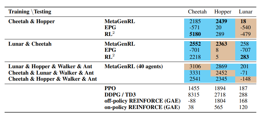
The authors trained the meta algorithm on the tasks in Cyan and tested on the tasks in brown
The big takeaway for me is that these strategies still definitively do not work (they’re worse than just directly learning the problem directly, by a long shot).
However, this algorithm definitely works more than the other meta-RL algorithms, which is promising.
To be slightly less sassy, the algorithm technically outperforms REINFORCE with GAE, which I would consider to be a pretty weak baseline. The competitive baselines are PPO and DDPG, of which it performs roughly equally to PPO and gets beaten pretty badly by DDPG. This is actually pretty encouraging, and the news only gets more encouraging, because their performance actually improves pretty substantially when they include more tasks. To me, this suggests that it legitimately is getting leverage out of the generality of more environments.
Future Directions & General Thoughts
I actually think that this idea is really encouraging and it makes a lot of sense. While this method doesn’t explicitly address any criticisms of existing algorithms, it’s very possible that it learns to do important things like propagating rewards backwards through time better than current methods. Right now, it takes \(100\) gradient steps before any action’s Advantage, Q-value, what have you, are affected by rewards received \(100\) timesteps down the line, which seems pretty excessive to me. This algorithm could learn to leverage that.
I think, for this algorithm to really make an impact though, I think we would need to see two things (besides just a performance increase). First, I would definitely want to see the performance of the algorithm on more tasks : can it actually beat algorithms like DDPG if given like 20 tasks? Probably not, but it would be good to get an idea how quickly the rewards of adding more tasks diminish.
Second, I think that the computation of the second derivative is likely prohibitive. Right now, the learned loss doesn’t generalize over multiple action cardinalities (meaning you need a separate model for a task with 5 actions versus 4 actions if you apply it in a discrete setting). That means that you would need to train separate models for each of those tasks, and I think that this algorithm is very likely extremely expensive. If it could either get rid of the 2nd order derivative (which would make it cheaper to train) or become more invariant (which allows it to be reused), I think it could be a lot more impactful.