
Hamiltonian Generative Networks
02 September 2020
Recent work, including Hamiltonian Neural Networks, Recurrent Independent Mechanisms & Visual Interaction Networks have made strides by applying basic principles from physics to their model structure. This work builds on the first of these Hamiltonian Networks to learn physical dynamics directly from pixels. The authors further apply this to predict future pixels, resulting in a generative model based on invertible flow.
Authors
- Peter Toth (Res. Eng. - DeepMind)
- Danilo J. Rezende (Sen. Staff. Res. Sci. - DeepMind)
- Andrew Jaegle (Res. Sci. - DeepMind)
- Sebastien Recaniere (Staff. Res. Eng. - DeepMind)
- Aleksander Botev (Res. Sci. - DeepMind)
- Irina Higgins (Sen. Res. Sci. - DeepMind)
ArXiV: https://arxiv.org/pdf/1909.13789.pdf
Background
Researchers have been using machine learning for prediction for a long, long time. One major domain therein is the video prediction, where the model first views a number of frames and then most predict futures frames. Many different types of models have been applied to this effect, with techniques ranging from visual flow to generative adversarial networks. Typically, the performance of these models degrades as they are forced to predict further and further in to the future, with visuals often becoming either less crisp or more erratic. Additionally, many of these methods can be very computationally expensive.
At it’s core, video prediction typically consists of predictions about videos containing real-world objects. Under this interpretation, one possible avenue is to try to extract the objects from an image, model the dynamics of the objects, then render the objects to an image that becomes the next prediction in the video sequence.
Core Idea
One of the core equations in physics is the idea of the Hamiltonian, an equation which relates the velocity and position of an object. Generally speaking, if \(\vec{q}\) is a vector representing the object’s position and \(\vec{p}\) represents the object’s momentum, then the following identity holds:
\[\frac{d \vec{q}}{dt} = \frac{\partial \mathcal{H}}{\partial \vec{p}}, \quad \frac{d \vec{p}}{dt} = - \frac{\partial \mathcal{H}}{\partial \vec{q}}\]where \(\mathcal{H}(p, q)\) is the Hamiltonian for the system. Different systems are characterized by different Hamiltonian equations, but this relationship holds in a wide number of scenarios for different Hamiltonian equations. The big idea of this paper is that, if we can learn the Hamiltonian for a system, then we can take it’s derivative to find \(\frac{d \vec{q}}{dt}\) and \(\frac{d \vec{p}}{dt}\). If we know the derivatives of \(p\) and \(q\), we can use classic numerical methods (e.g. Euler integration) to predict the values of \(p\) and \(q\) forward and backward in time.
The general flow of the model is :
- Estimate \(p\) and \(q\) from a video sequence
- Estimate \(dp\) and \(dq\) by deriving the Hamiltonian.
- Use numerical integration to predict the next timestep.
- Use deconvolutional techniques to render these values to an image.
Note that steps 2 & 3 may be repeated to derive predictions further in the future.
Details
There are a LOT of details here, so I’ll try to keep it to the core essence.
1. Extracting \(p\) and \(q\) from video sequence
The first part of this is extremely similar to the first part of a VAE. We want to take in some sequence of images and encode them in a latent space, where the encodings resemble some probability distribution. Namely, the authors learn some function \(q_\phi(z|\vec{x}_0, \vec{x}_1, ..., \vec{x}_n)\) where \(\vec{x}_i\) is the \(i^{th}\) image in the sequence s.t.
\[E_{\vec{x}_0, \vec{x}_1, ..., \vec{x}_n}\Big[KL(q_\phi(z|\vec{x}_0, \vec{x}_1, ..., \vec{x}_n) \| p(z))\Big]\]is minimized. In principle, \(p(z)\) could be any probability distribution over the vector space. In practice, people usually choose \(p(z) = \mathcal{N}(0, I)\), and this paper is no different. Afterwards, \(z\) is fed in to another embedding network \(f_\psi\), which outputs the physical state \(s\). Half of the variables are arbitrarily assigned to represent \(p\) and half are arbitrarily assigned to represent \(q\).
2. Deriving the Hamiltonian
The authors introduce the Hamiltonian network \(H_\gamma\), parameterized by, you guessed it, \(\gamma\). In the original HNN paper, the Hamiltonian network was given an explicit loss to minimize, which were inspired by the physical properties of the Hamiltonian. Here, however, the Hamiltonian network is trained in an end-to-end function. It’s output is meaningless, only the derivative of the output has intrinsic meaning. Deriving the Hamiltonian with respect ot its inputs is trivial using basic autodifferentiation tools like Tensorflow & PyTorch.
3. Using numerical integration for prediction
Given the aforementioned identities \(\frac{d \vec{q}}{dt} = \frac{\partial \mathcal{H}}{\partial \vec{p}}, \quad \frac{d \vec{p}}{dt} = - \frac{\partial \mathcal{H}}{\partial \vec{q}}\), we are now able to obtain estimates of \(\frac{d\vec{q}}{dt}\) and \(\frac{d\vec{p}}{dt}\) by deriving our Hamiltonian network with respect to it inputs. This makes the problem a numerical integration problem, where
\[q_{t+h} = q_t + h\frac{d\vec{q_t}}{dt}\] \[p_{t+h} = p_t + h\frac{d\vec{p_t}}{dt}\]It’s fairly straightforward to extend this forward in time by simply replacing \(q_t\) with \(q_{t+h}\) (the same is true for \(p\)). This process is called Euler integration. In practice, the authors use a slightly different algorithm called leapfrom integration, where you alternate between updating \(p\) and \(q\) instead of doing both each timestep. Additionally, you can also model backwards in time by simply using \(-h\) instead of \(h\). Conveniently, you’ll notice that both versions are fully differentiable, which leads us to…
4. Rendering the Image
For any given timestep, we can concatenate the \(p\) and \(q\) vectors for each timestep. Notably, only \(q\), the vector containing position, is necessary to render the image - \(p\), the momentum, is only used for prediction. The decoder network, \(d_\theta(q_t)\) is a deconvolutional network.
This entire process is trained end-to-end with the following loss function:
\[L(\phi, \psi, \gamma, \theta; \vec{x}_0, \vec{x}_1, ..., \vec{x}_n) = \frac{1}{T+1} \sum^T_{t=0}\Big[E_{q_\phi(z|\vec{x}_0, \vec{x}_1, ..., \vec{x}_n)}[log(p_{\psi, \gamma, \theta}(x_t|q_t))]\Big] - KL(q_\theta(z)\|p(z))\]Which is really long. We can separate it in to two parts. The second part just encourages the encodings \(z\) to mimic the normal distribution, as we described in section 1. Because each part of this model is invertible, we can assign a probability to each possible video frame in the predicted sequence. Conveniently, this lets us estimate the predicted probability of the actual observation. Our goal is to make the model assign high probability to the frames that are actually in the dataset.
A schematic of the whole process is below:
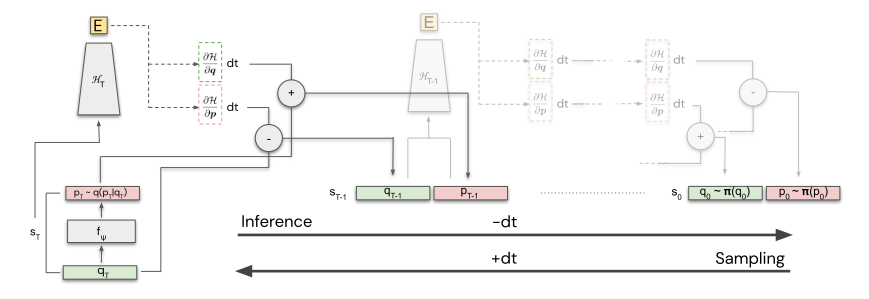
sliiiightly convoluted
Experiments
The authors test on basically the same problems that the original HNN paper did, except that they test primarily on pixels, without any ground-truth knowledge about position or momentum. Of note, the original HNN also included some experiments learning directly from pixels, with a model that they call PixelHNN. The authors compare to that model, as well as performing several ablation studies.
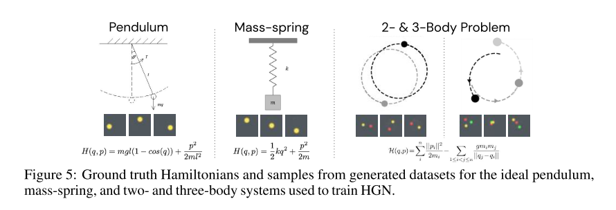
The 4 environments are shown below, and are pretty self-explanatory.
The authors convincingly outperform the original PixelHNN.
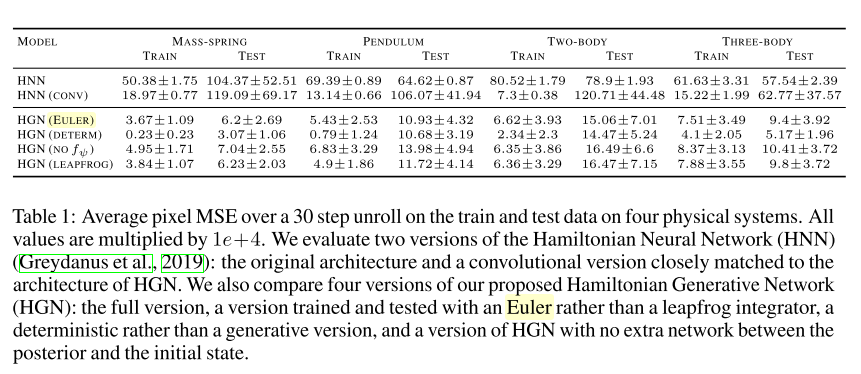
interestingly, the authors make their model non-deterministic, but it appears that the deterministic version performs better.
The authors also include several experiments showing that their model is able to learn multimodal densities, which is reassuring.
Future Directions & General Thoughts
There are a lot of useful things that this paper does. I appreciate that it generalizes the idea of the Hamiltonian to successfully use it in an end-to-end manner. I think that the general approach of applying lessons in physics to modeling is very useful, but I also think that it’s likely useful to make these lessons as broad as possible, which this paper does, by getting rid of a lot of the specifics that were present in the original model.
That being said, there are a number of things I’m relatively unconvinced by. Many of the design choices are somewhat unmotivated, most notably in the initial encoding scheme (which, of note, is where the authors also did the most ablation studies). I appreciate that their design choices generally help, but I’m not as convinced that these choices will be applicable in other domains. Looking through the appendix, there are also a number of pretty specific hyperparameters in their networks, which give me questions.
Finally, I think that it would be useful to see baselines besides HNNs and I would be interested in seeing whether or not this method can scale to non-toy domains.