(Algorithmic Alignment): What Can Neural Networks Reason About?
24 August 2020
In an (algorithmically) ideal world, machine learning would be able to complete all of the tasks that traditional programs do. However, it’s no secret that there are some functions that neural networks are able to learn better than others. This paper seeks to quantify this intuition and provides a new concept called ‘algorithmic alignment’.
Authors
- Keyulu Xu (PhD Cand. - CSAIL, MIT)
- Jingling Li (PhD Cand. - UMaryland, UMIACS)
- Mozhi Zhang (PhD Cand. - UMaryland, Jordan Boyd-Graber’s Lab)
- Simon S. Du (Asst. Prof. - UWash)
- Ken-ichi Kawarabayashi (Prof., JST ERATO Kawarabayashi Proj., National Institute of Informatics)
- Stefanie Jegelka (Assoc. Prof. - CSAIL, MIT)
ArXiV: https://openreview.net/pdf?id=rJxbJeHFPS
Background
Similar to what we saw in Neuro-Symbolic VQA, there’s been a fair amount of work in getting machine-learning models (let’s be real, neural nets) to solve reasoning problems.
People have established a fair number of different architectures to try to solve these problems, but their performance can vary heavily by task (and often be brittle).
For context, the authors provide several reasoning tasks that neural networks can be applied to:
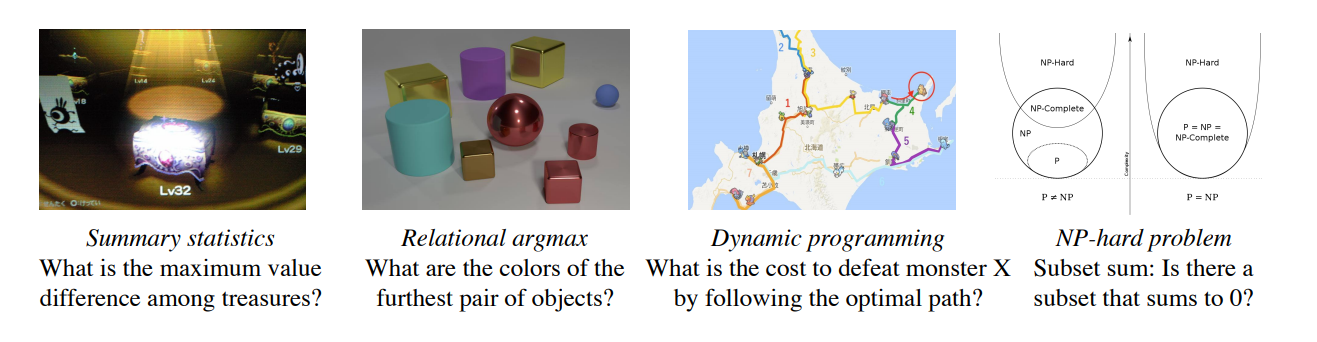
I appreciate that these guys managed to work Pokemon in to an academic paper.
The problems above are divided into four groups as follows:
- Summary Statistics : These problems involve aggregating information about a properties of the input.
- Relational Argmax : Compare relationships, and then use that information to compute an answer
- Dynamic Programming : You probably know dynamic programming - the one sentence definition is solving smaller sub-problems and memoizing them.
- NP-Hard : Ummm…. let’s just say these are really, really hard. Our current encryption methods rely on these problems not being solveable in any reasonable amount of time \(^*\).
The authors note that while basic Multi-Layer Perceptrons have had a lot of difficulties with these problems, Deep Set Networks do substantially better, and GNNs often do better still.
Core Idea
At a high-level, this trend makes sense : a lot of these problems can be viewed through the lens of objects interacting with each other. From this perspective, you would expect every object to have roughly the same dynamics, but to interact with each other dynamically, which is what GNNs allow. But this is still a pretty fuzzy intuition, how can we make it more formal?
Well, first, what do we mean when we say a network architecture is able to ‘solve’ a type of problem? If we let the network have infinite data, the problem’s pretty trivial - Neural Nets are known to be universal function approximators, so an MLP could solve any problem with enough capacity, compute and data. You could reasonably limit the models on any of those three axes, but this paper looks at the problem through the lense of data - how much data do we need to generalize well?
Again, we’re brought back to the question of ‘solving’ a problem. Here, we turn to the Probably Approximately Correct (PAC) framework, which has just the most evasive name possible. In general, we can say that a model is \(\epsilon, \delta\) PAC if our error (however you compute that) only ever exceeds \(\epsilon\) on \(\delta\)% of inputs. So, the probability that we’re correct is \(1-\delta\) and we’ll say we’re correct if our approximation is less than \(\epsilon\) off of the true target.
Here, you can then ask how much data an algorithm needs to be PAC, which turns out to be a fairly lengthy equation.
Either way, the authors turn their attention to the problem of learning to approximate solutions for which there exists a ‘correct’ solution.
Let’s say that we have some ‘correct’ algorithm \(g\), and we’re trying to learn a model \(\mathcal{N}\) to approximate it.
We could theoretically swap out the submodules of our network with some other functions.
For instance, in a GNN, instead of using a neural network for message passing, we could use a hard-coded function.
If it’s possible to find a function that causes our GNN to become identical to the ‘correct’ algorithm, then the problem is only as hard as finding that function.

We're looking for relations like this.
Details
OK, math time.
First, to formally define PAC. We’ll stick with all of the definitions above, adding a dataset-size variable \(M\), which controls the number of samples that we draw from the distribution \(\mathcal{D}\) with labels and observations. If we sample i.i.d. M times from \(\mathcal{D}\) to get our dataset \(X, Y\), we can train our model on it \(f = \mathcal{A}(X, Y)\). Here, \(\mathcal{A}\) is just the training process and \(f\) is the resulting model. Then we say that \(\mathcal{D}\) is \(M, \delta, \epsilon\) learnable if
\[P_{x \sim \mathcal{D}}\Big[\|f(x) - g(x)\| \leq \epsilon] \geq 1 - \delta\]Basically, \(\delta, \epsilon\) are strictness parameters and \(M\) is how much data we’re giving the training algorithm. From this, we can say that the sample complexity of an algorithm \(\mathcal{A}\) is the lowest \(M\) such that \(\mathcal{A}\) is \(M, \delta, \epsilon\) learnable. Holding \(\epsilon\) and \(\delta\) constant, we’re basically asking how much data do I need to give algorithm \(\mathcal{A}\) so that it can solve \(\mathcal{D}\)?
The author’s primary contribution is this:
Let’s say that our network \(\mathcal{N}\) can be split into \(n\) modules \(\mathcal{N}_i\). If there are functions \(f_i\) that we can replace each \(\mathcal{N}_i\) with so that the neural network exactly mimics the correct solution, then we’ll say that \(\mathcal{N}\) is algorithmically aligned with \(g\). In this case, the difficulty of learning the whole model is equal to the difficulty of learning the hardest part.
For a sanity check, let’s consider the case where we call \(\mathcal{N}\) one big module \(\mathcal{N}_0\). In that case, this theorem tells us that learning \(\mathcal{N}_0\) should be just as hard as solving \(f_0\). However, because \(\mathcal{N}_0 \equiv \mathcal{N}\), then \(f_0 \equiv g\), where \(g\) is our original ‘correct’ algorithm. Essentially, we just recovered the identity - breaking the problem in to 1 subproblem results in a subproblem that’s just as hard as the original.
The last result here is estimating the sample complexity for an MLP? The authors only prove the scenario for the case where you train one layer at a time, but I’d be willing to bet that you get a similar result in generality. The actual equation isn’t super illuminating, so I’ll list the key takeaways:
- The sample complexity of the whole model is grows with the maximum of the complexity of its inner parts.
- If you approximate the target function as a sum of polynomials (think Taylor expansion), then the sample complexity grows exponentially with the highest power of that polynomial.
- The sample complexity increases proportional to \(1/\epsilon^2\)
- In general, higher coefficients in the polynomial function make it harder to learn
The authors also note that an aligned GNN of \(l\) nodes takes \(O(l^2)\) less data than an MLP of the same input if it is aligned well.
Experiments
To validate all of this theory, the authors run a number of experiments.
They test MLPs, Set Networks and GNNs on the above 4 problems shown, and report their test accuracy.
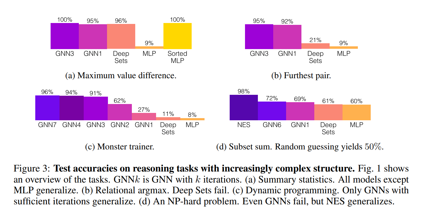
You’ll notice that the MLP does pretty terribly on all of the tasks.
When finding the maximum value difference, which is a simple set aggregation problem, the deep sets network does just as well as GNNs.
On the harder problems, GNNs have algorithmic alignment, so they do pretty well.
The obvious exception is subset-sum, which is NP-hard. Here, GNNs do surprisingly well, but not incredibly. Subset-sum involves identifying whether there is a subset of numbers in a list that sum to 0s. You probably noticed the best performing model is one called NES. NES stands for neural exhaustive search. In this model, the authors basically take random subsets of the list and throw them in to a neural network, which basically has to check whether or not they sum to 0. This is pretty clearly aligned with the brute-force solution to subset sum, so it performs quite well (although I’m sure that it is, computationally speaking, abominable to run).
Future Directions & General Thoughts
The results of this paper basically say what you would expect them to. If your model lines up with the target problem, it does better. For instance, with their result that a GNN learns \(O(l^2)\) faster than an MLP when aligned makes sense - it has \(O(l^2)\) fewer parameters. There are a lot of other intuitive things that this paper shows, but I think that they are very much worth showing.
There are a lot of very unintuitive results in mathematics (for instance, here’s one that always boggles my mind). Additionally, this can give theoretical justification for a lot of design problems going forward, and can help us filter out bad ideas or build better ideas. This paper took a little bit to understand, and I think it will take longer to fully digest, but I see a lot of value here.